A Short Intro of Intel Advanced Matrix Extensions (AMX)
Based on my talk at QCon San Francisco 2024
Watch the talk: Maximizing Deep Learning Performance on CPUs using Modern Architectures — includes slides, video, and full transcript.
Introduction
When people think about deep learning acceleration, GPUs are what typically come to mind. But in my experience helping teams deploy AI workloads across cloud, on-premises, and hybrid environments, a huge number of production workloads still run on CPUs. Sometimes it’s availability — GPUs are hard to come by, or you’d rather reserve them for training large language models. Sometimes the models are inherently memory-bandwidth-bound. And sometimes the economics just work out better on CPUs.
And CPUs have gotten really good at this. When Llama 3.1 was released, published benchmarks showed ~1 token per 20 milliseconds on a compressed model running on a 5th-generation Xeon server. Not GPU. CPU.
Whether you’re already deploying on CPU or doing feasibility analysis to see if you can, I want to share what I’ve learned about squeezing maximum performance out of modern CPU hardware — so you can make an informed decision. This post breaks down into four parts: Why should I care? → What does it solve? → How does it solve it? → How do I leverage it?
What AI Workloads Actually Run on CPUs?
Not everything needs a GPU. Many production workloads run on CPUs, including:
- Smaller Transformer models: BERT, RoBERTa, DistilBERT, MobileBERT, TinyBERT
- Lightweight CNNs: MobileNet, SqueezeNet, EfficientNet
- Recurrent Neural Networks (RNNs): LSTM and GRU-based models
- Recommendation models: almost everything except heavy-rankers
- Tree-based models: XGBoost, Random Forest, Gradient Boosting Machines
For these workloads, CPU inference is often more cost-effective and simpler to deploy than spinning up GPU instances. And as low-precision computing techniques improve, even LLMs are becoming viable on CPU — quantized models are your friend.
GEMMs Dominate the Runtime
At the heart of nearly every deep learning model lies General Matrix Multiplication (GEMM). The numbers are striking:
| Model Family | GEMM % of Runtime |
|---|---|
| Transformers (BERT, GPT) | ~70% |
| CNNs | ~50–60% |
| RNNs | ~40–60% |
Whatever model you are running on the surface — transformer, CNN, RNN — eventually what you’re doing on the hardware is spending a lot of cycles doing matrix multiplication. If you want to make deep learning faster on CPUs, optimizing GEMM is where the biggest wins are.
From Naive to Fast: The MatMul Optimization Journey
Step 1: Naive Matrix Multiplication
The textbook triple-nested loop. Simple, correct, and slow.
1
2
3
4
5
6
7
8
9
10
11
12
// M = N = K = 1024
// Runtime: 730ms

for (int m = 0; m < M; m++) {
    for (int n = 0; n < N; n++) {
        float sum = 0.0f;
        for (int k = 0; k < K; k++) {
            sum += A[m * K + k] * B[k * N + n];
        }
        C[m * N + n] = sum;
    }
}
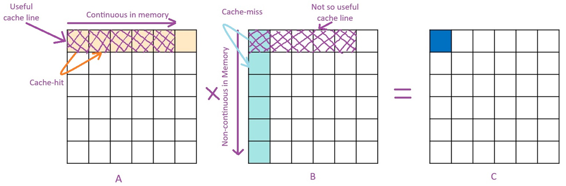 Figure: naive loop order fetches a full cache line from B but uses only one element before jumping rows.
This accesses matrix B in a column-wise pattern — terrible for cache performance since data is stored row-major. When you fetch a data element from B, the hardware brings an entire cache line into L1 (typically 64 bytes — 16 floats). But in this loop order, you only use one element from that cache line before jumping to the next row. All those prefetched elements go to waste. You paid the cost to bring them into L1, but they’re evicted before they’re ever used.
Step 2: Reorder the Loops
A simple loop reorder gives us a 5.6x speedup — with zero algorithmic changes:
1
2
3
4
5
6
7
8
9
10
// M = N = K = 1024
// Runtime: 130ms

for (int m = 0; m < M; m++) {
    for (int k = 0; k < K; k++) {
        for (int n = 0; n < N; n++) {
            C[m * N + n] += A[m * K + k] * B[k * N + n];
        }
    }
}
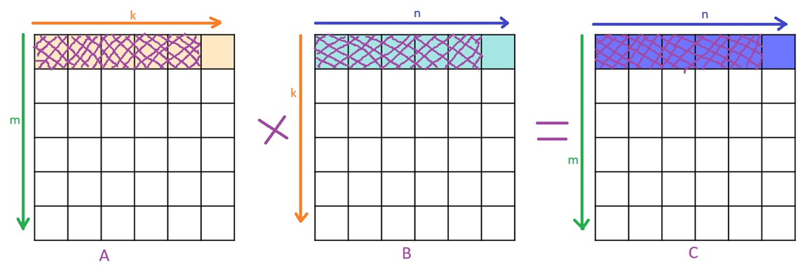 Figure: reordered loop streams through B with stride-1 access, using every element in the cache line.
By swapping the K and N loop order, we get consecutive memory access on all three matrices. The inner loop now streams through both B and C with stride-1 access. Every element fetched into cache actually gets used — far more cache-friendly.
Step 3: Tiled (Blocked) Matrix Multiplication
Tiling breaks the matrices into smaller blocks that fit in cache:
1
2
3
4
5
6
7
8
9
10
11
12
13
14
15
16
17
// M = N = K = 1024, T = 128
// Runtime: 89ms

for (int m = 0; m < M; m += T) {
    for (int n = 0; n < N; n += T) {
        for (int k = 0; k < K; k += T) {
            // Multiply T x T sub-blocks
            for (int mt = m; mt < std::min(m+T, M); ++mt) {
                for (int kt = k; kt < std::min(k+T, K); ++kt) {
                    for (int nt = n; nt < std::min(n+T, N); ++nt) {
                        C[mt*N+nt] += A[mt*K+kt] * B[kt*N+nt];
                    }
                }
            }
        }
    }
}
This improves temporal locality — we reuse data while it’s still in cache.
1
2
3
4
5
6
7
8
9
Core
 ↓
L1 / L2
 ↓
Distributed LLC (mesh)
 ↓
(optional) HBM (on-package via EMIB)
 ↓
DDR (via integrated memory controllers)
Figure: Modern CPU memory hierarchy — registers (< 1 ns), L1 cache (~1 ns, ~48 KB), L2 cache (~4 ns, ~2 MB), L3 cache (~10 ns, ~100 MB), DRAM (~50 ns). Tiling targets keeping working sets in L1/L2; AMX tiles live in registers.
The Reality: Data Locality Is Everything
The progression from 730ms → 130ms → 89ms illustrates a fundamental truth: spatial and temporal data locality dominates performance. But there’s more to the story:
- Implementing efficient tiled matmul is much more complicated than the simple version above
- Tiling is not cache-agnostic — you need to tune tile sizes to your specific cache hierarchy
- Multi-tiered caches (L1/L2/L3) complicate the optimal blocking strategy
- Vector processing units (SIMD) open up additional optimization opportunities
For reference, NumPy achieves 13ms for the same 1024×1024 multiply — under the hood it delegates to an optimized BLAS library (typically oneMKL or OpenBLAS). We’re still 7× away from that optimal solution, and there are literally teams of hundreds of engineers at every major company working full-time to optimize GEMM kernels.
The key takeaway from this exercise: for better performance, you want a large amount of useful data as close to the CPU as possible. Not just any data — data you’ll actually use.
Key insight: What’s better than having 2D tiles in L1 cache? Having 2D tiles in registers. You can load 1 kilobyte of data into a single register.
This is exactly the idea behind Intel AMX.
Low Precision Computation: Why It Matters
Before diving into AMX, it’s worth understanding why low-precision computation is so important for deep learning:
| Format | Structure | Use Case |
|---|---|---|
| FP32 | 1 sign + 8-bit exponent + 23-bit mantissa | Default for training and inference |
| BF16 | 1 sign + 8-bit exponent + 7-bit mantissa | Training and inference |
| FP16 | 1 sign + 5-bit exponent + 10-bit mantissa | Inference (limited range) |
| INT8 | 8-bit signed/unsigned | Inference |
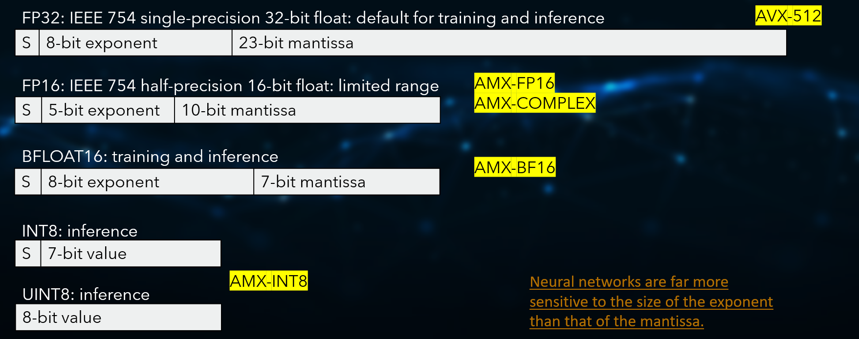 Figure: Bit-field breakdown of numeric formats used in deep learning. BF16 keeps the same 8-bit exponent as FP32 (preserving dynamic range) but truncates the mantissa from 23 to 7 bits.
A critical observation: neural networks are far more sensitive to the size of the exponent than the mantissa. This is why BFloat16 (which keeps the FP32 exponent range but truncates the mantissa) works so well for training, and why INT8 quantization is effective for inference.
AMX: 2D Registers Meet Matrix Multiply
Advanced Matrix Extensions (AMX), introduced with the 4th Gen Xeon Scalable processors (Sapphire Rapids), is the ISA extension I’ve found most impactful for CPU-based deep learning. It brings two key innovations:
1. Tiles: 2D Register Files
Instead of 1D vector registers (like AVX-512’s 512-bit registers), AMX introduces tile registers — 2D blocks that can store larger chunks of matrix data.
2. TMUL: Tile Matrix Multiply Unit
A dedicated accelerator that computes matrix multiplications on entire tiles in a single operation. Under the hood, TMUL is a 2D systolic array of Fused Multiply-Add (FMA) ALUs — it propagates data from tile A and tile B through the array, multiplying and accumulating into tile C. This dedicated silicon is present on every single core.
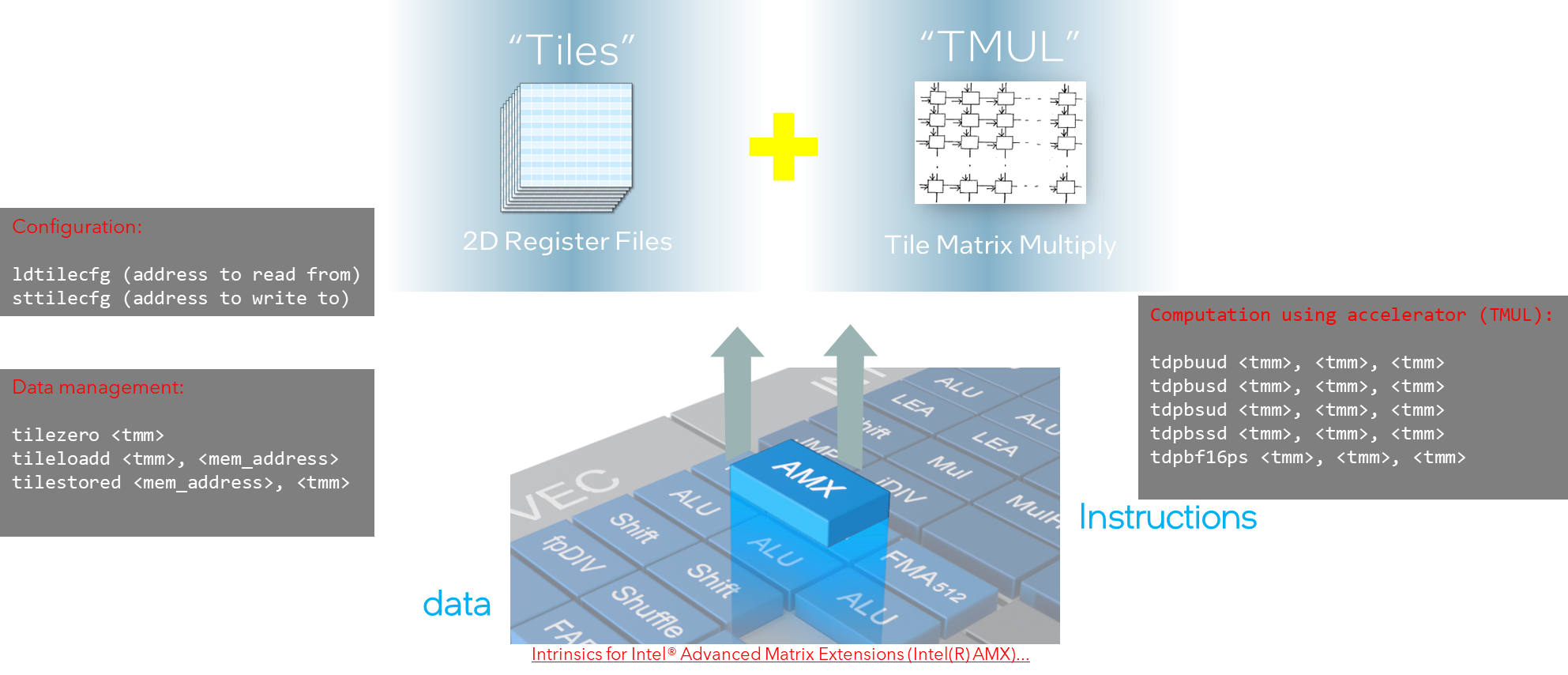 Figure: The 8 AMX tile registers (tmm0–tmm7). Each tile holds up to 16 rows × 64 bytes — fitting 16×64 INT8 values or 16×32 BF16 values. Underutilized tiles are zero-padded.
Tile Specifications
- 8 tiles available in total (tmm0–tmm7)
- Each tile: maximum 16 rows × 64 bytes
- One tile can fit:
- 16 × 64 INT8 values, or
- 16 × 32 BFloat16 values
- Accumulation is done in INT32 (for INT8 inputs) or FP32 (for BF16 inputs)
- Underutilized tiles are zero-padded
What this means in practice:
- Multiply two 16×64 INT8 tiles → get a 16×16 INT32 result
- Multiply two 16×32 BF16 tiles → get a 16×16 FP32 result
Programming AMX: Step by Step
Prerequisites
You need:
- 4th Gen (or newer) Xeon Scalable processor — Sapphire Rapids or later. On AWS, look for M7i, R7i, C7i instances. On GCP looks for c3 instances.
- Linux Kernel 5.16+ — that’s when the AMX intrinsics were introduced.
Verify AMX support in your CPU flags (look for amx_tile, amx_bf16, amx_int8):
1
lscpu | grep -E "amx_bf16|amx_tile|amx_int8"
Step 1: Enable AMX
For power efficiency, AMX is disabled by default. If your code needs AMX, you must make a system call to request access to the tile data resources:
1
2
3
4
5
6
7
8
9
static bool set_tiledata_use() {
    if (syscall(SYS_arch_prctl, ARCH_REQ_XCOMP_PERM, XFEATURE_XTILEDATA)) {
        printf("\n Fail to do XFEATURE_XTILEDATA \n\n");
        return false;
    } else {
        printf("\n TILE DATA USE SET - OK \n\n");
        return true;
    }
}
Step 2: Configure Tiles
Define the tile configuration — palette, row counts, and column byte widths. The palette_id must be 1 when initializing tiles. The start_row field is for fault tolerance — if an AMX instruction fails, the hardware knows where to resume fetching data:
1
2
3
4
5
6
7
8
9
10
11
12
13
14
15
16
17
18
19
typedef struct __tile_config {
    uint8_t palette_id;      // byte 1
    uint8_t start_row;       // byte 2
    uint8_t reserved_0[14];  // bytes 2-15
    uint16_t colsb[16];     // bytes 16-47
    uint8_t rows[16];       // bytes 48-63
} __tilecfg;

static void init_tile_config(__tilecfg *tileinfo) {
    tileinfo->palette_id = 1;
    tileinfo->start_row = 0;

    // tmm0 = C[M][N] (int32), tmm1 = A[M][K] (int8), tmm2 = B[K][N] (int8)
    for (int i = 0; i < 3; ++i) {
        tileinfo->colsb[i] = 64;
        tileinfo->rows[i] = 16;
    }
    _tile_loadconfig(tileinfo);
}
Step 3: Load Data into Tiles
1
2
3
4
5
6
7
int8_t  A[1024];   // 16 x 64
int8_t  B[1024];   // 16 x 64
int32_t C[256];    // 16 x 16

_tile_loadd(1, A, STRIDE);  // Load A into tmm1
_tile_loadd(2, B, STRIDE);  // Load B into tmm2
_tile_loadd(0, C, STRIDE);  // Load C into tmm0
Step 4: Compute and Store
1
2
3
4
5
// Compute dot-product of INT8 tiles, accumulate into INT32
_tile_dpbssd(0, 1, 2);

// Store result back to memory
_tile_stored(0, result, STRIDE);
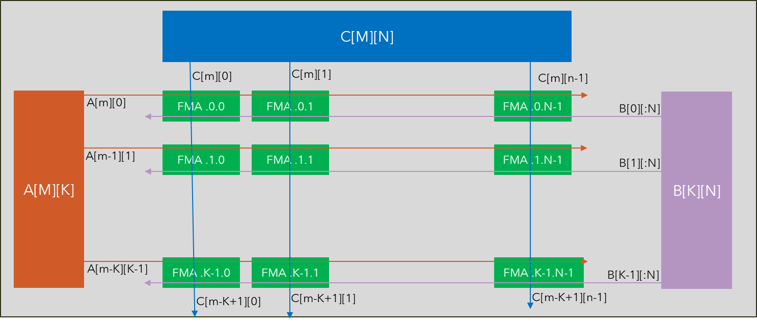 Figure: The TMUL unit is a 2D systolic array of FMA ALUs. Data from tile A propagates horizontally, tile B vertically, and results accumulate in tile C. Each FMA computes C[m][n] += A[m][k] × B[k][n].
The inner computation follows:
1
2
3
4
for m < M:       // time steps
  for k < K:     // grid height
    for n < N:   // SIMD dimension
      C[m][n] += Mul(A[m][k], B[k][n])
Supported AMX Instructions (4th & 5th Gen Xeon)
| Instruction | Description |
|---|---|
tdpbf16ps | BF16 dot-product → FP32 accumulation |
tdpbuud | Unsigned × Unsigned INT8 → INT32 |
tdpbusd | Unsigned × Signed INT8 → INT32 |
tdpbsud | Signed × Unsigned INT8 → INT32 |
tdpbssd | Signed × Signed INT8 → INT32 |
6th Gen Xeons add AMX-FP16 and AMX-COMPLEX support.
The nice thing about this architecture is that it’s extensible. As new low-precision formats gain traction — FP8, INT4, whatever comes next — native hardware support can be added in future CPU generations without changing the programming model.
Tiling Larger Matrices with AMX
Real matrices are larger than 16×64. We need to tile the computation across the full matrix, using the 8 available tile registers strategically.
For a blocked 2×2 decomposition:
1
2
A = [A11 A12]    B = [B11 B12]    C = [C11 C12]
    [A21 A22]        [B21 B22]        [C21 C22]
The computation becomes:
1
2
3
4
C11 += A11 * B11 + A12 * B21
C12 += A11 * B12 + A12 * B22
C21 += A21 * B11 + A22 * B21
C22 += A21 * B12 + A22 * B22
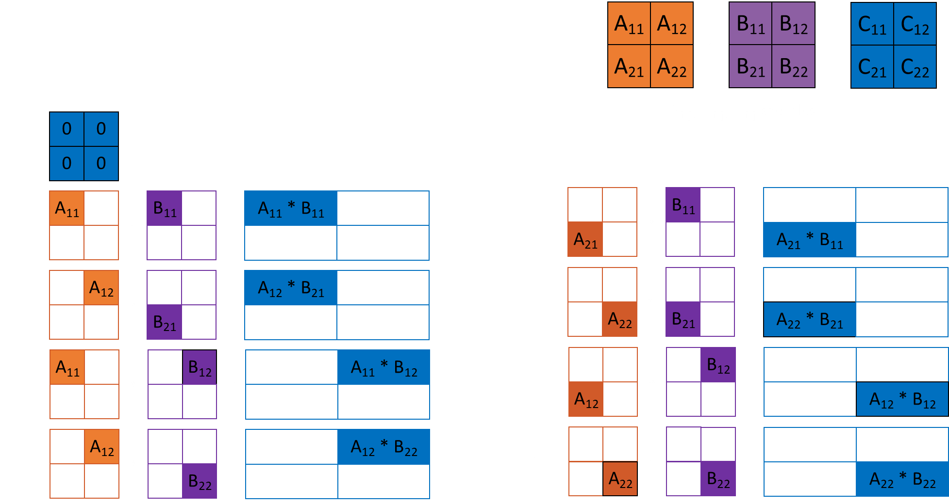 Figure: Mapping of the 8 tile registers for a 2×2 blocked GEMM. tmm0–tmm3 hold the four C output tiles. tmm4–tmm5 are loaded with A sub-blocks, tmm6–tmm7 with B sub-blocks (transposed). Arrows show data flow from RAM through tiles to the TMUL unit.
The 8 tile registers are mapped as:
- tmm0–tmm3: C tiles (C11, C12, C21, C22)
- tmm4–tmm5: A tiles (loaded as needed)
- tmm6–tmm7: B tiles (loaded transposed)
The execution flow: zero the C tiles → load A/B sub-blocks from RAM → execute tile multiplies → store C tiles back to memory. This pattern repeats as we sweep across the full matrix dimensions.
Performance Impact: AMX in Practice
The throughput improvements over AVX-512 FP32 are substantial:
| Model | AMX-BF16 | AMX-INT8 |
|---|---|---|
| DistilBERT | 5.4× | 5.9× |
| ResNet-50 | 6.8× | 10.8× |
| Mask R-CNN (ResNet50) | 7.5× | 11.6× |
| EfficientNet-B0 | 1.2× | 1.5× |
| BERT-base-cased | 5.7× | 8.4× |
Platform: Xeon Platinum 8580, PyTorch 2.4.0. These are my own measurements, not official vendor benchmarks.
The theoretical throughput tells the story: up to 1024 BF16 ops/cycle and 2048 INT8 ops/cycle with AMX, compared to just 64 FP32 ops/cycle with AVX-512.
How Do I Take Advantage of AMX?
The answer depends on your role:
If You Write Custom Kernels or Compilers
You’ll need to work with the tile intrinsics or TMUL instructions directly. This is really only necessary if you’re building novel primitives that existing libraries don’t cover.
If You Work on Framework Backends
Integrate AMX-enabled libraries like oneDNN or oneMKL as your compute backend. These handle the ISA-specific codegen so you don’t have to.
If You’re a Data Scientist or ML Engineer
Just use a recent version of your framework — PyTorch, TensorFlow, or serving stacks like Triton, TorchServe, vLLM. They already dispatch to AMX kernels when the hardware supports it.
If You Want to Push Further
Tools like Intel Neural Compressor (accuracy-aware quantization), OpenVINO (end-to-end optimization + serving), and IPEX (Intel Extension for PyTorch) can squeeze out additional performance. I’ve found these particularly useful when the default framework path leaves performance on the table.
Using AMX in Frameworks
Here’s the good news: you probably don’t need to do any of the above manually. If you use a modern framework on a supported CPU, AMX gets used whenever possible.
PyTorch
PyTorch uses oneDNN by default on CPU. For AMX-BF16, just run your model with Auto Mixed Precision:
1
2
with torch.cpu.amp.autocast():
    output = model(input)
For AMX-INT8, quantize your model and run it — PyTorch will automatically dispatch to AMX-INT8 kernels via oneDNN:
1
2
3
4
quantized_model = torch.quantization.quantize_dynamic(
    model, {torch.nn.Linear}, dtype=torch.qint8
)
output = quantized_model(input)
This works with both torch.compile and TorchScript-exported models.
TensorFlow
After TensorFlow 2.10, oneDNN is used by default on CPU. Enable AMX-BF16 by setting:
1
2
3
import os
os.environ['TF_ENABLE_ONEDNN_OPTS'] = '1'
os.environ['DNNL_MAX_CPU_ISA'] = 'AMX_BF16'
Going Beyond the Defaults
If the built-in framework support isn’t hitting the performance you need, there are additional tools I’ve found useful in practice:
- IPEX (Intel Extension for PyTorch) — Contains optimizations not yet upstreamed to mainline PyTorch. I’ve seen meaningful gains on certain model architectures.
- Intel Extension for TensorFlow — Same idea for the TF ecosystem.
- Intel Neural Compressor — Accuracy-aware model compression. The key feature: you can set a tolerance (“no more than 1% accuracy loss”) and it searches for the best quantization config within that budget. Saves a lot of manual tuning.
- Intel Extension for Transformers — Focused compression for transformer models. Supports BF16, INT8, INT4, even INT2.
- OpenVINO Toolkit — End-to-end: model compression plus deployment with its own Model Server. Worth evaluating if you want a single stack for optimization and serving.
What’s Next
This post covered the why — why modern ISA extensions like AMX are a game-changer for CPU-based deep learning. But you don’t have to program AMX tiles by hand. In Part 2, we’ll look at how to use oneDNN’s Batch-Reduce GEMM (BRGeMM) — a production-grade, ISA-tuned kernel that abstracts away the hardware details while giving you near-peak performance out of the box.
Conclusion
The journey from a 730ms naive matmul to AMX-accelerated computation is a masterclass in hardware-software co-design:
- Loop reordering (730ms → 130ms): Respect memory access patterns
- Tiling (130ms → 89ms): Fit working sets in cache
- Optimized BLAS (~13ms): Multi-level blocking, packing, SIMD vectorization
- AMX (5–11× over AVX-512): 2D register files + dedicated matrix multiply hardware
Modern CPUs are far more capable for deep learning than many assume. With AMX, current-generation Xeon processors can deliver significant inference throughput — especially when combined with quantization to INT8 or BF16 precision. The key is understanding the memory hierarchy and leveraging the right hardware features at each level.
One practical tip: if you have a small model, use a larger batch size so the GEMM operations fill all 16 rows of the AMX tiles. With batch size 1, your GEMM becomes a matrix-vector multiply (GEMV), and you’ll waste most of the tile resources — only 1 of 16 rows gets used. AMX works best when you can keep those tiles full.
Bibek Bhattarai QCon San Francisco 2024 | Watch the talk
Additional readings
- Why GEMM is at the heart of deep learning – https://petewarden.com/2015/04/20/why-gemm-is-at-the-heart-of-deep-learning/
- BFloat16: The secret to high performance on Cloud TPUs – https://cloud.google.com/blog/products/ai-machine-learning/bfloat16-the-secret-to-high-performance-on-cloud-tpus
- Intel® Intrinsics Guide – https://www.intel.com/content/www/us/en/docs/intrinsics-guide/index.html#!=undefined&techs=AMX
- Tiled Matrix Multiplication – https://penny-xu.github.io/blog/tiled-matrix-multiplication
- Intel® 64 and IA-32 Architectures Software Developer Manuals – https://www.intel.com/content/www/us/en/developer/articles/technical/intel-sdm.html